Uniformly Distributed Loads

This group of load types is used to apply on beam elements forces and moments distributed over the whole element length. Generally, the direction of loading may be specified either in the global coordinate system or in the local element coordinate system.

Per default, all UDL load types are line loads (option Load/Unit length) related to the element length (force per unit length) (option Real length). In accordance with the deformation method theory for beams, this distributed line load is internally transformed into forces and moments acting on the nodes.

Alternatively, the UDL load types may be specified to be

Projected loads	load intensity related to the projection of the element length	(option Projection)
Surface loads	load intensity related to an area (length × width or depth)	(options Load mult. by CS width and Load mult. by CS depth)
Nodal loads	transformation to the start and end nodes without moments	(option Nodal load)

Option	Description
Projection	Projected loads are related to the length of projection of the element normal to the load direction rather, than to the real element length. This can for instance be used for defining distributed snow or wind loads, where the load intensity is measured per unit length of the element projection. The intensity would be the depth of snow or the dynamic pressure of the wind; the projected element length is measured in a plane perpendicular to the direction of loading.
Load mult. by CS width	The entered load intensities Qx, Qy, Qz are surface loads related to the product of the element length and the cross-section width (defined as the sum z1+z2 of the cross-section properties z1 and z2). Note that in this context the unit [Length(structure)] is considered for the cross-section width, although z1 and z2 are given in the GUI in [Length(CS)]. The unit of the surface load will therefore always be the force unit divided by the square of the length unit specified as [Length(structure)].
Load mult. by CS depth	The entered load intensities Qx, Qy, Qz are surface loads related to the product of the element length and the cross-section depth (defined as the sum y1+y2 of the cross-section properties y1 and y2). Note that in this context the unit [Length(structure)] is considered for the cross-section depth, although y1 and y2 are given in the GUI in [Length(CS)]. The unit of the surface load will therefore always be the force unit divided by the square of the length unit specified as [Length(structure)]. Note: When cross-section widths or depths at the two element ends differ, the respective line load values will be evaluated, and the average value will be used as uniformly distributed over the element length. Note that any lateral eccentricity of the surface loading – due to either y1 and y2 or z1 and z2 being different – is not automatically considered. The entered load intensities Qx, Qy, Qz are surface loads related to the product of the element length and the cross-section width or depth, assumed acting concentrically on the elements if no eccentricities are specified by the user.
Nodal Load	An UDL specified as nodal load will be transformed into two equivalent point loads acting on the start and end points of the element. This means, that the rigid constraint moments theoretically arising at the element ends will not be taken into account. Any nodal moments arising due to eccentric connections between element ends and node will however be considered. This option is not applicable for Surface loads.

Related reference
Uniform Concentric Element Load Uniform Eccentric Element Load Self weight (load and/or mass)

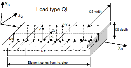
Uniform concentric element load – load types QG, QL

QG	Uniformly distributed concentric element load defined in terms of components (Qx, Qy, Qz) in global coordinate directions. Concentric UDL defined in terms of components in global directions
QL	Uniformly distributed concentric element load defined in terms of components (Qx, Qy, Qz) in the local element coordinate system and acting over the whole element length. Concentric UDL defined in terms of components in local directions

Uniform eccentric element load – load types QEXG, QEXL, QEYG, QEYL, QEZG, QEZL

QEXG	Eccentric UDL (global) - Uniformly distributed eccentric element load in terms of components in global coordinate directions and acting over the whole element length. The eccentricity is defined in the local system with reference to the cross-section centroid (from the centroid to the load application line).
QEXL	Eccentric UDL (local) - Uniformly distributed eccentric element load in terms of components in local coordinate directions and acting over the whole element length. The eccentricity is defined in the local coordinate system with reference to the cross-section centroid (from the centroid to the load application line).
QEYG	Eccentric UDL in global direction acting on the whole length of the element.
QEYL	Eccentric UDL in local direction acting on the whole length of the element.

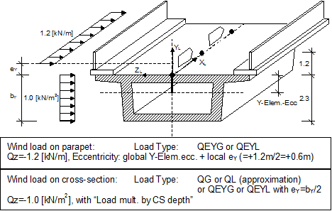
QEYG and QEYL are similar to QEXG and QEXL respectively, but the specified load eccentricity in Y-direction (Ey) is not related to the element axis but to the connection line between the two cross-section reference points. The Y-component of the cross-section eccentricity is automatically added internally. Ez remains related to the element axis.

Application example 1: superimposed dead load - walkway

Example for using vertical eccentric distributed loading

Note: Per default, load eccentricities are defined in the local coordinate system with the origin in the cross-section centroid (QEXG, QEXL). Using the load types QEYG, QEYL allows for relating the y-component of the load eccentricity being related to the cross-section reference point (the z component remains related to the element axis). For the load types QEZG, QEZL this applies analogously in local z-direction.

QEZG	Eccentric UDL in global direction acting on the whole length of the element.
QEZL	Eccentric UDL in local direction acting on the whole length of the element.

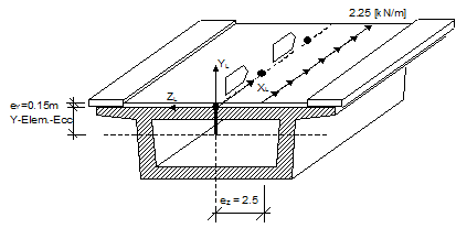
QEZG and QEZL are similar to QEXG and QEXL, but the specified load eccentricity in Z-direction (Ez) is not related to the element axis but to the connection line between the two cross-section reference points. The Z-component of the cross-section eccentricity is automatically added internally. Ey remains related to the element axis.

Application example 2: Transverse wind load on the structure

Example for using horizontal eccentric distributed loading

Application example 3: Braking force in accordance with AUSTRIAN Standard

Design force according to the code is the worst of:

30% of the heaviest vehicle as point load
10 kN * Roadway width in m
5% of total uniform load as uniform load

All loads are acting at the top of the pavement

Example:

Length L=34+44+44+34=156 m Width of the roadway = 9 m.

Heaviest vehicle 250 kN Uniform traffic load = 5 kN/m²

--> 0.3 * 250 = 75 kN

--> 10.0 * 9.0 = 90 kN

--> 9.0*156*0.05*5= 351 kN =>decisive force

=> qx = 351/156 = 2.25 kN/m or 0.25 kN/m²

Braking force on an eccentric lane

Self weight – load types G, G0, GM

G	Self-weight – load and mass.
G0	Self-weight just as load; like G, but no mass matrix terms are generated.
GM	Self-weight just as mass; like G, but no load terms (only mass matrix) are generated.

These load types use the cross-section area Ax for creating the corresponding line load intensities and/or distributed mass intensities respectively. The input value Gam specifies the specific weight to be considered. The material parameter Gamma of the element material is used if no value Gam is specified (Gam=0.0). The entered direction vector (Rx, Ry, Rz) is internally normalized and characterizes the load direction.

The corresponding mass terms are calculated by dividing the load intensity value Ax×Gam by the gravity constant g specified in Recalc > Dynamic. The direction vector is not used for calculating the self-weight mass terms (same value for all 3 directions).

Note: The average cross-section area is taken if the cross-sections at the element start and element end differ. This average area is multiplied by the specific weight, giving the actual UDL value.

Application example: Static earthquake loading

Assumption: Two Load Sets have to be applied in 2 separate Load Cases for simulating either an earthquake in the longitudinal direction or an earthquake in lateral direction. This is only an application example and might be different in different codes or cases.

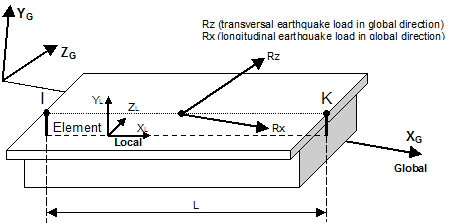
Modeling earthquake loading with load type Self-weight acting in horizontal directions

Loadset1 - Static earthquake in longitudinal direction: Rx=1.00, Ry=0, Rz=0 density g=25kN/m³(100% of the self-weight in x-direction); Loadcase1 with Loadset1 and constant factor of 0.05 (5% of Load Set 2 in x-direction)

Loadset2 - Static earthquake in transversal direction: Rx=0, Ry=0, Rz=1.00 density g=1.25kN/m³ (5% of the self-weight in z-direction), Loadcase2 with Loadset2 and with a constant factor of 1.00.

Self-weight of active part of composite elements – types GPA, GPA0, GPAM

These load types are related to composite structures only. In principle, GPA, GPA0 and GPAM calculate the self-weight of the considered elements like G, G0 and GM respectively (being considered as loading and mass, only as loading, or only as mass; see load type self weight).

For normal elements without composite cross-section, GPA, GPA0 and GPAM will be equivalent to G, G0 and GM respectively. For composite elements, these load types allow for applying the self-weight on the individual parts rather, than specifying it for the active composite element characterizing the current structural stiffness. This allows for instance for using the material parameter Gamma (specific weight) rather than a specific user specified fictitious specific weight Gam of the composite element.

Self-weight of inactive parts of composite elements – GPI, GPI0, GPIM

These load types are related to composite structures only. In principle, GPI, GPI0 and GPIM calculate the self-weight of the considered elements like G, G0 and GM respectively (being considered as loading and mass, only as loading, or only as mass; see load type self weight).

For normal elements without composite cross-section, GPI, GPI0 and GPIM will be equivalent to G, G0 and GM respectively. For composite structures, these load types allow for applying the self-weight of inactive parts of the final composite cross-section on the currently active part characterizing the structural stiffness. This can for instance advantageously be used for specifying the wet concrete load of partial elements applied before they become active.